stanford cs336 学习笔记
课程的目的
想要真正在 AI 行业做出创新,就必须了解其底层原理,而不是只是调参数、调 API。
AI 大厂正在垄断并封闭先进的 AI 技术,必须学习底层原理,才能复刻这些成果。
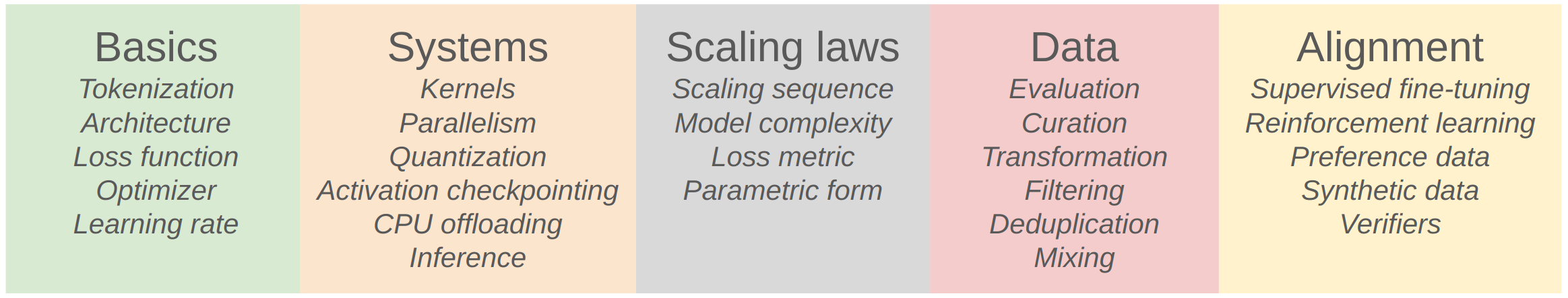
在课程中,学生将亲手训练 <1 B 参数模型:数据抓取 → 清洗 →Tokenizer→Transformer→ 训练 → 评估。通过实操体会调度、并行、混精、省显存等工程细节,把平常抽象调用的网络结构拉回到可自主控制修改的范围。
Byte-Pair Encoding (BPE) Tokenizer
The Unicode Standard
unicode 标准给世界所有语言的每个字符指定了一个对应的数字编号
Problem (unicode1): Understanding Unicode (1 point)
(a) What Unicode character does chr(0) return?
1
'\x00'
(b) How does this character’s string representation (
__repr__()) differ from its printed representation?1
__repr__() 会返回一个便于程序调试的信息,而print返回一个便于人类可读的信息。比如 chr(0) 的内容就无法用 print 打印,但可以用 repr 实现按 hex 显示(c) What happens when this character occurs in text? It may be helpful to play around with the following in your Python interpreter and see if it matches your expectations:
1
2
3
4
>>> chr(0)
>>> print(chr(0))
>>> "this is a test" + chr(0) + "string"
>>> print("this is a test" + chr(0) + "string")
1
chr(0)返回的是不可视的字符,所以无法用print()打印
Unicode Encodings
通过 utf-8 或其他编码规则,可以将自然语言编码成计算机能处理的字节串。
Problem (unicode2): Unicode Encodings (3 points)
(a) What are some reasons to prefer training our tokenizer on UTF-8 encoded bytes, rather than UTF-16 or UTF-32? It may be helpful to compare the output of these encodings for various input strings.
1
大部分的都是英文字母,utf-8 长度更短
(b) Consider the following (incorrect) function, which is intended to decode a UTF-8 byte string into a Unicode string. Why is this function incorrect? Provide an example of an input byte string that yields incorrect results.
1
2
3
4
def decode_utf8_bytes_to_str_wrong(bytestring: bytes):
  return "".join([bytes([b]).decode("utf-8") for b in bytestring])
>>> decode_utf8_bytes_to_str_wrong("hello".encode("utf-8"))
  'hello'
1
2
3
4
5
6
utf-8是变长的,不能拆分为单字节解码
decode_utf8_bytes_to_str_wrong("你好".encode("utf-8"))
Traceback (most recent call last):
  File "<stdin>", line 1, in <module>
  File "<stdin>", line 2, in decode_utf8_bytes_to_str_wrong
UnicodeDecodeError: 'utf-8' codec can't decode byte 0xe4 in position 0: unexpected end of data
(c) Give a two byte sequence that does not decode to any Unicode character(s).
1
0xFF 0xFF
Subword Tokenization
字节级(byte-level)分词(Tokenization)可以彻底解决词表外(OOV)问题,但会显著拉长输入序列长度,从而增加计算开销并加剧长程依赖,导致模型训练变慢、建模更困难。
子词(subword)分词是介于词级和字节级之间的折中方案:通过使用更大的词表来压缩字节序列长度。字节级分词的基础词表只有 256 个字节值,而子词分词会把高频出现的字节序列(如 the)合并成一个 token,从而减少序列长度。BPE(Byte-Pair Encoding)通过反复合并最常见的字节对来构建这些子词单元,使频繁出现的词或片段逐渐成为单个 token。基于 BPE 的子词分词器在保持良好 OOV 处理能力的同时,显著缩短序列长度;构建其词表的过程称为 BPE tokenizer 的训练。
BPE Tokenizer Training
训练 BPE 的三个步骤:
Vocabulary initialization(词表初始化)
词表是从 token 到整型 id 的映射表。这个表在训练前的默认值非常简单,就是每个 byte(ascii) 到对应的数字,比如
'a'(0x61) -> 97,共 256 条。Pre-tokenization(预标记)
先提取出所有的单词(特殊组合),统计每个单词出现的次数,然后再匹配每个字母字节的个数及其邻近关系
常用的预标记正则:
1
PAT = r"""'(?:[sdmt]|ll|ve|re)| ?\p{L}+| ?\p{N}+| ?[^\s\p{L}\p{N}]+|\s+(?!\S)|\s+"""
(?:...)问号和冒号放在括号里表示这个捕获组仅分组,而不产生分组编号,无法使用$1之类的方式访问'(?:[sdmt]|ll|ve|re)表示匹配所有'和后面的特定词,比如'll(I’ll)、'm(I’m)、't(don’t)等(所有格)- ` ?\p{L}+
表示匹配 0 到 1 个空格,然后\p{L}+` 表示按照 L 规则的 Unicode 类型匹配字符,可以匹配所有字母,结果就是一个空格加一个单词(除了段落开头的那个单词是没空格的) - ` ?\p{N}+` 同上匹配空格,表示按照 N 规则匹配,可以匹配所有数字,结果就是一个空格加一串数字
- ` ?[^\s\p{L}\p{N}]+` 同上匹配空格,然后不匹配所有的空格、字母、数字,其实就是匹配所有标点符号和表情符号、运算符等
\s+(?!\S)表示匹配多个连续的空格,但后面不能有非空格(\S),所以只能匹配段落末尾的连续空格,中间的空格尾部都会跟字母或者数字。\s+表示匹配多个连续的空格
这个正则相当于是英语语句的基本语法,比如用空格分隔单词,用
'm这种表示所有格(possessive)或缩写最后会得到一张预标记表:每一条的格式是[预标记,数量],也就是每个词出现的次数: 比如
{"the": 20, "+": 2, "dog": 5, "'ll": 1}Compute BPE merges(计算 BPE 合并)
根据预标记表,统计词表中的哪两个 token (第一次处理这些词都是初始化词表中单个字节的字符)能拼在一起(连续出现的概率较高)
比如一个句子中有很多的
the,则t h和h e两个组合出现概率高,就会拼在一起作为一个新的 token 加入词表。此时词表中同时有tethhe重复这个操作,大概率
th将会和e拼接为the加入词表。此时词表中同时有tethhethe
Experimenting with BPE Tokenizer Training
现在用 TinyStories 数据集训练一个 BPE 模型
Pre-tokenization 比较耗时,可以用已有的分块并行化处理函数:
Problem (train_bpe): BPE Tokenizer Training (15 points)
使用 uv run pytest tests/test_train_bpe.py 运行测试
核心思路:
- 先找到所有的仅两个字符组成的pair,放入 pair 池中
- 找到出现次数最多的pair(可以使用最大堆),将其移出池,加入 merges 列表,找到其在所有文本中的位置(可以保存pair位置表) a. 生成新pair: 将其前一个token和其本身组成pair,将其与其后一个token组成pair,都加入池中。(可以保存pair组合表,需要知道前一个后一个token是否是多个字符的组合) b. 删除老pair: 将其前一个token和其第一个元素组成的pair,将其第二个元素与其后一个token组成的pair,都移出池
- 重复 2 过程,直到 merges 列表数量达到要求
1
2
3
4
5
6
7
8
9
10
11
12
13
14
15
16
17
18
19
20
21
22
23
24
25
26
27
28
29
30
31
32
33
34
35
36
37
38
39
40
41
42
43
44
45
46
47
48
49
50
51
52
53
54
55
56
57
58
59
60
61
62
63
64
65
66
67
68
69
70
71
72
73
74
75
76
77
78
79
80
81
82
83
84
85
86
87
88
89
90
91
92
93
94
95
96
97
98
99
100
101
102
103
104
105
106
107
108
109
def run_train_bpe(
    input_path: str | os.PathLike,
    vocab_size: int,
    special_tokens: list[str],
    **kwargs,
) -> tuple[dict[int, bytes], list[tuple[bytes, bytes]]]:
    """Given the path to an input corpus, run train a BPE tokenizer and
    output its vocabulary and merges.

    Args:
        input_path (str | os.PathLike): Path to BPE tokenizer training data.
        vocab_size (int): Total number of items in the tokenizer's vocabulary (including special tokens).
        special_tokens (list[str]): A list of string special tokens to be added to the tokenizer vocabulary.
            These strings will never be split into multiple tokens, and will always be
            kept as a single token. If these special tokens occur in the `input_path`,
            they are treated as any other string.

    Returns:
        tuple[dict[int, bytes], list[tuple[bytes, bytes]]]:
            vocab:
                The trained tokenizer vocabulary, a mapping from int (token ID in the vocabulary)
                to bytes (token bytes)
            merges:
                BPE merges. Each list item is a tuple of bytes (<token1>, <token2>),
                representing that <token1> was merged with <token2>.
                Merges are ordered by order of creation.
    """
    vocab = {}
    merges = []
    # vocabulary 初始化
    vocab_index = 0
    for special_token in special_tokens:
        vocab[vocab_index] = special_token.encode()
        vocab_index = vocab_index + 1
    for i in range(0,256):
        vocab[vocab_index] = bytes([i])
        vocab_index = vocab_index + 1

    with open(input_path, "br", encoding="utf-8") as f:
        content = f.read()
    # 去掉特殊字符(拆分文章)
    special_tokens_pattern = "|".join(map(re.escape, special_tokens))
    parts = re.split(special_tokens_pattern, content)
    # A. Pre-tokenization
    pre_tokens = {}
    PAT = re.compile(rb"""'(?:[sdmt]|ll|ve|re)| ?\p{L}+| ?\p{N}+| ?[^\s\p{L}\p{N}]+|\s+(?!\S)|\s+""")
    for part in parts:
        matches = re.finditer(PAT, part)
        for val in matches:
            pre_token = val.group()
            pre_tokens[pre_token] = pre_tokens.get(pre_token, 0) + 1
    # B. Compute BPE merges
    token_pairs = {}
    # 1. 提取所有单字节的pair
    for pre_token, count in pre_tokens.items():
        for i in range(len(pre_token)-1):
            token_pair = (pre_token[i].to_bytes(), pre_token[i+1].to_bytes())
            token_pairs[token_pair] = token_pairs.get(token_pair, 0) + count

    # 2. 根据已经有的pair更新计数
    while True:
        max_token_pair = tuple()
        max_token_count = 0
        for token_pair, count in token_pairs.items():
            if count > max_token_count:
                exsited = False
                for merge_pair in merges:
                    if merge_pair[0] + merge_pair[1] == token_pair[0] + token_pair[1]:
                        exsited = True
                        break
                if exsited:
                    continue
                max_token_count = count
                max_token_pair = token_pair
        token_pairs[max_token_pair] = 0
        vocab[vocab_index] = max_token_pair[0] + max_token_pair[1]
        vocab_index = vocab_index + 1
        merges.append(max_token_pair)

        if vocab_index >= vocab_size:
            break
        for pre_token, count in pre_tokens.items():
            pos = 0
            while True:
                max_token_bytes = max_token_pair[0] + max_token_pair[1]
                pos = pre_token.find(max_token_bytes, pos)
                if pos == -1:
                    break
                if pos >= 1:
                    token_pair = (pre_token[pos - 1:pos], max_token_bytes)
                    token_pairs[token_pair] = token_pairs.get(token_pair, 0) + count
                if pos + len(max_token_bytes) < len(pre_token):
                    token_pair = (max_token_bytes, pre_token[pos + len(max_token_bytes):pos + len(max_token_bytes)+1])
                    token_pairs[token_pair] = token_pairs.get(token_pair, 0) + count

                for merge_pair in merges:
                    merge_pair_token = merge_pair[0] + merge_pair[1]
                    if pos >= len(merge_pair_token):
                        if pre_token[pos - len(merge_pair_token):pos] == merge_pair_token:
                            token_pair = (merge_pair_token, max_token_bytes)
                            token_pairs[token_pair] = token_pairs.get(token_pair, 0) + count
                    if pos < len(pre_token) - len(merge_pair_token):
                        if pre_token[pos + len(max_token_bytes):pos + len(max_token_bytes)+len(merge_pair_token)] == merge_pair_token:
                            token_pair = (max_token_bytes, merge_pair_token)
                            token_pairs[token_pair] = token_pairs.get(token_pair, 0) + count

                pos = pos + len(max_token_bytes)

    return (vocab, merges)
BPE Tokenizer: Encoding and Decoding
Encoding text
在上一节中,我们通过训练获得了一张 vocabulary 表,假设是这样的:{0: b' ', 1: b'a', 2: b'c', 3: b'e', 4: b'h', 5: b't', 6: b'th', 7: b' c', 8: b' a', 9: b'the', 10: b' at'}
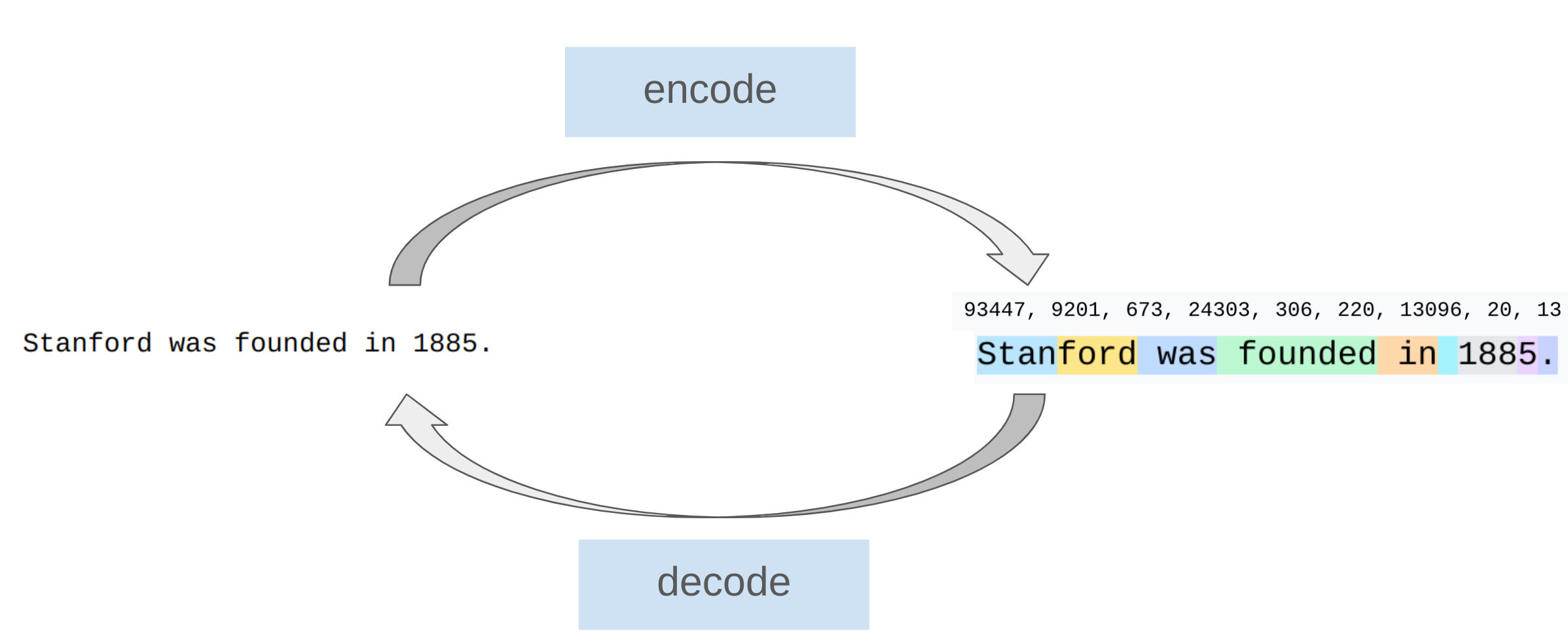
对于一篇新的文章,我们用这张 vocabulary 表对其进行 encoding 操作:
- 首先还是 Pre-tokenization,将其拆分为一个个单词,比如
['the', ' cat', ' ate'] - 然后对于每一个单词,查找 vocabulary 获取适合其的拆分,比如
'the'拆分为[the],' cat'拆分为[ c][a][t],[' ate']拆分为[ at][e] - 拆分后用 vocabulary 中对应的序号表示这个 token,就能得到
[9, 7, 1, 5, 10, 3],完成 encoding
Decoding text
就是 Encoding 的反过程,通过 [9, 7, 1, 5, 10, 3] 获得 the cat ate。
Transformer Language Model Architecture
本章节介绍从零开始构建一个 transformer language model
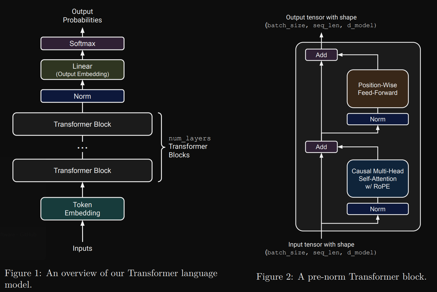
Transformer LM
Token Embeddings
首先用之前生成的 vocabulary 表对输入的文本进行 encoding 操作,将其分为若干 token 并变成 token ID 序列,最后生成的矩阵就是 (batch_size, sequence_size),在 LLM 模型中,输入文本被拆分为一个个句子, batch_size 就是句子的数量,sequence_size 就是句子的 token ID 序列长度(每句长度相同,不足的填充 padding):
1
2
3
4
5
6
sentences = [
    "I love machine learning",      # 样本1 -> [12, 2342, 5342, 223, 334, 223]
    "Transformers are amazing",     # 样本2
    "Deep learning is fun",         # 样本3
    "AI is changing the world"      # 样本4
]
然后使用 embedding模型将每个 token 转为一个向量(分特征),此时矩阵变为 (batch_size, sequence_size, d_model), d_model 就是 embedding 模型的输出长度
Pre-norm Transformer Block
嵌入之后的向量序列,会被送入多个结构完全相同的神经网络层进行深度处理。这些层依次对数据进行加工,逐渐提取和组合出越来越复杂的特征。
对于 decode-only 的 transformer 架构,每一个神经网络层的结构都相同,输入输入输出都是 (batch_size, sequence_size, d_model),每一层都会执行自注意力(融合上下文,计算每个 token 间的联系)和feed-forward前馈网络(深度处理)操作
Output Normalization and Embedding
对输出结果的归一化和向量化
将 (batch_size, sequence_size, d_model) 的输出转变为 predicted next-token logits(vocabulary表中每个token的得分,得分高的被预测为下一个 token)
Remark: Batching, Einsum and Efficient Computation
Transformer 中的大部分计算都是以”批量操作”的方式进行的,将相同操作应用于多个独立但结构相同的输入单元上。有 3 个维度的批量操作:
批处理维度
每个批次中,同时处理多个样本(句子),使用完全相同的参数和流程
序列维度
一个序列中的每个 token 在 RMSNorm 和前馈网络中的处理逻辑(位置无关操作)都是相同的
attention heads 维度
多个注意力头是并行计算的
建议使用 einsum 来进行矩阵操作:
示例1:
1
2
3
4
5
6
7
8
9
10
11
12
13
14
15
import torch
from einops import rearrange, einsum

## Basic implementation
Y = D @ A.T
# Hard to tell the input and output shapes and what they mean.
# What shapes can D and A have, and do any of these have unexpected behavior?

## Einsum is self-documenting and robust
#                            D              A     ->         Y
Y = einsum(D, A, "batch sequence d_in, d_out d_in -> batch sequence d_out")
# 自动对 A 做了转置,变成 (d_in d_out) 形状,从而可以和 D 进行点乘

## Or, a batched version where D can have any leading dimensions but A is constrained.
Y = einsum(D, A, "... d_in, d_out d_in -> ... d_out")
示例2:
1
2
3
4
5
6
7
8
9
10
11
12
13
14
15
16
17
18
# We have a batch of images, and for each image we want to generate 10 dimmed versions based on some scaling factor:
# 假设要对每张图片使用不同的校色参数生成10份校色后副本
images = torch.randn(64, 128, 128, 3) # (batch, height, width, channel), 64张 128x128,rgb图像
dim_by = torch.linspace(start=0.0, end=1.0, steps=10) # 生成长度为10的向量: [0.0 0.1111 ... 0.8889 1.0]

## Reshape and multiply
dim_value = rearrange(dim_by, "dim_value -> 1 dim_value 1 1 1") # 改变维度形状,将一维张量扩展为5维
images_rearr = rearrange(images, "b height width channel -> b 1 height width channel") # 将4维张量变为5维
dimmed_images = images_rearr * dim_value # 进行广播后做乘法

## 以上三个语句可以用一条语句表示
dimmed_images = einsum(
    images, dim_by,
    "batch height width channel, dim_value -> batch dim_value height width channel"
)

# 注意:[batch dim_value height width channel] 和 [batch height width channel dim_value] 含义不同,但在数学上是等价的。
# 前者含义为当前图片的当前 dim 下有这么些像素及每个像素的rgb值,后者含义为当前图片的每个像素的每个channel有这么些 dim
示例3:
1
2
3
4
5
6
7
8
9
10
11
12
13
14
15
16
17
18
19
20
21
22
23
24
25
26
27
28
29
30
31
32
33
34
35
36
37
38
39
40
41
42
43
44
45
46
47
48
49
50
51
52
53
# Suppose we have a batch of images represented as a tensor of shape (batch, height, width,
# channel), and we want to perform a linear transformation across all pixels of the image, but this
# transformation should happen independently for each channel. Our linear transformation is
# represented as a matrix B of shape (height × width, height × width).
channels_last = torch.randn(64, 32, 32, 3) # (batch, height, width, channel)
B = torch.randn(32*32, 32*32)
# 1. Rearrange an image tensor for mixing across all pixels
# 形状变化: [64, 32, 32, 3] → [64, 1024, 3]
# 将32×32的二维网格展平为1024的一维序列
channels_last_flat = channels_last.view(
    -1, channels_last.size(1) * channels_last.size(2), channels_last.size(3)
)
# 形状变化: [64, 1024, 3] → [64, 3, 1024]
# 现在每个通道的所有像素是连续存储的
channels_first_flat = channels_last_flat.transpose(1, 2)
# 矩阵乘法: [64, 3, 1024] @ [1024, 1024] → [64, 3, 1024]
# 对每个通道的1024个像素进行线性混合
channels_first_flat_transformed = channels_first_flat @ B.T
# 形状变化: [64, 3, 1024] → [64, 1024, 3],恢复顺序
channels_last_flat_transformed = channels_first_flat_transformed.transpose(1, 2)

# 形状变化: [64, 1024, 3] → [64, 32, 32, 3],恢复维度
channels_last_transformed = channels_last_flat_transformed.view(*channels_last.shape)
# 2. Instead, using einops:
height = width = 32
## Rearrange replaces clunky torch view + transpose
# 展平、交换顺序
channels_first = rearrange(
channels_last,
    "batch height width channel -> batch channel (height width)"
)
# 和B的转置做点乘(线性变换)
channels_first_transformed = einsum(
channels_first, B,
    "batch channel pixel_in, pixel_out pixel_in -> batch channel pixel_out"
)
# 恢复形状
channels_last_transformed = rearrange(
channels_first_transformed,
    "batch channel (height width) -> batch height width channel",
    height=height, width=width
)
# 3. Or, if you’re feeling crazy: all in one go using einx.dot (einx equivalent of einops.einsum)
height = width = 32
channels_last_transformed = einx.dot(
    "batch row_in col_in channel, (row_out col_out) (row_in col_in)"
    "-> batch row_out col_out channel",
    channels_last, B,
    col_in=width, col_out=width
)
# The first implementation here could be improved by placing comments before and after to indicate
# what the input and output shapes are, but this is clunky and susceptible to bugs. With einsum
# notation, documentation is implementation!
Mathematical Notation and Memory Ordering
向量的表达形式和内存顺序
- 行向量:(1, d)
- 列向量: (d, 1)
行向量和列向量通过转置就能互转,本质是一样的,但是计算机一般更倾向于处理行向量,因为张量的每一行的每个元素在计算机中是内存连续的,但行与行之间的内存没有必然联系。
但是在数学中,列向量用的比较多,本教程的数学表达式更倾向于使用列向量,但读者应该知道写代码时优先使用行向量。另外如果使用 einsum 做计算,即使用列向量也没什么影响,会自动转为行向量提高性能的。
Basic Building Blocks: Linear and Embedding Modules
Parameter Initialization
合理的初始化参数能避免训练过程中梯度消失或爆炸等问题:
Linear weights:
$\mathcal{N}(\mu = 0,\ \sigma^2 = \frac{2}{d_{\text{in}} + d_{\text{out}}})$ truncated at $[-3\sigma, 3\sigma]$Embedding:
$\mathcal{N}(\mu = 0,\ \sigma^2 = 1)$ truncated at $[-3, 3]$.方差为1,均值为0,所有
[-3,3]外的值直接截断为 -3 或 3。RMSNorm: 1
用 torch.nn.init.trunc_normal_ 进行初始化
Linear Module
\[y = Wx\]现代大语言模型都不再包含偏置(bias)
作业:Implement a Linear class that inherits from torch.nn.Module and performs a linear transformation. Your implementation should follow the interface of PyTorch’s built-in nn.Linear module, except for not having a bias argument or parameter
继承自nn.Module
1
2
3
4
5
6
7
8
9
10
11
12
13
14
15
16
17
18
19
20
21
22
23
24
25
26
27
28
29
30
31
32
33
34
35
36
37
38
39
40
41
42
43
44
45
46
47
48
49
50
51
52
53
54
55
56
57
58
59
60
61
import torch
import torch.nn as nn
import torch.nn.functional as F
import math
from einops import rearrange, einsum


class Linear(torch.nn.Module):
    """Linear layer without bias, following modern LLM conventions."""

    def __init__(self, in_features: int, out_features: int, device=None, dtype=None):
        """
        Initialize a linear transformation module.

        Args:
            in_features: int, final dimension of the input
            out_features: int, final dimension of the output
            device: torch.device | None, device to store the parameters on
            dtype: torch.dtype | None, data type of the parameters
        """
        super().__init__()

        self.in_features = in_features
        self.out_features = out_features

        # Initialize weight parameter (W, not W^T for memory ordering reasons)
        # Shape: (out_features, in_features)
        self.W = torch.nn.Parameter(torch.empty(out_features, in_features, device=device, dtype=dtype))

        # Initialize weights using truncated normal distribution
        self._init_weights()

    def _init_weights(self):
        """Initialize weights using truncated normal distribution as specified."""
        # Calculate standard deviation for linear weights
        sigma = math.sqrt(2.0 / (self.in_features + self.out_features))

        # Calculate truncation bounds: [-3*sigma, 3*sigma]
        a = -3 * sigma
        b = 3 * sigma

        # Initialize weights with truncated normal distribution
        with torch.no_grad():
            torch.nn.init.trunc_normal_(self.W, mean=0.0, std=sigma, a=a, b=b)
        # 这里的with torch.no_grad():是一种防御性编程,防止这个初始化操作被意外加入梯度计算中

    def forward(self, x: torch.Tensor) -> torch.Tensor:
        """
        Apply the linear transformation to the input.

        Args:
            x: torch.Tensor, input tensor of shape (..., in_features)

        Returns:
            torch.Tensor, output tensor of shape (..., out_features)
        """
        # Use einsum for matrix multiplication
        # x shape: (..., in_features)
        # W shape: (out_features, in_features)
        # Output shape: (..., out_features)
        return einsum(self.W, x, "out in, ... in -> ... out")
Embedding Module
如上模型结构所述,Transformer 的第一层就是 Embedding 层,用于将 token ID 映射到 d_model 大小的向量空间,见Token Embeddings
作业:Implement the Embedding class that inherits from torch.nn.Module and performs an embedding lookup. Your implementation should follow the interface of PyTorch’s built-in nn.Embedding module.
1
2
3
4
5
6
7
8
9
10
11
12
13
14
15
16
17
18
19
20
21
22
23
24
class Embedding(torch.nn.Module):
    def __init__(self, num_embeddings, embedding_dim, device=None, dtype=None):
        """
        Initialize a Embedding transformation module.

        Args:
            num_embeddings: int Size of the vocabulary
            embedding_dim: int Dimension of the embedding vectors, i.e., dmodel
            device: torch.device | None = None Device to store the parameters on
            dtype: torch.dtype | None = None Data type of the parameters
        """
        super().__init__()

        self.vocab_size = num_embeddings
        self.d_model = embedding_dim
        self.W = torch.nn.Parameter(torch.empty(self.vocab_size, self.d_model, device=device, dtype=dtype))
        with torch.no_grad():
            torch.nn.init.trunc_normal_(self.W, mean=0.0, std=1, a=-3, b=3)

    def forward(self, token_ids: torch.Tensor) -> torch.Tensor:
        '''
        Lookup the embedding vectors for the given token IDs.
        '''
        return self.W[token_ids]
Pre-Norm Transformer Block
每个 transformer block 内有两层:
- multi-head self-attention mechanism
- position-wise feed-forward network
如上面架构图所示,每层之前都会做 Norm 操作,然后会进行残差连接
不过在最初的 transformer 中,Norm 是放在每次残差连接之后的,见此处,也就是每层的最后,后来研究发现,将 Norm 放在每个层的前面效果会更好。
Root Mean Square Layer Normalization
我们使用均方根归一化实现 Norm 层操作
\[RMSNorm(a_i) = \frac{a_i}{RMS(a)} g_i\]其中,$ RMS(a) = \sqrt{\frac{1}{d{\text{model}}} \sum{i=1}^{d_{\text{model}}} a_i^2 + \varepsilon} $,$g_i$ 是一个可学习的 “gain(增益)” 参数(总个数和 a 一样,为 d_model),$\varepsilon$ 是常量 $10^{-5}$
在计算过程中,要临时提升至 torch.float32 精度,最后结果要还原回原来的精度:
1
2
3
4
5
6
7
in_dtype = x.dtype
x = x.to(torch.float32)
# Your code here performing RMSNorm
...
result = ...
# Return the result in the original dtype
return result.to(in_dtype)
作业:Implement RMSNorm as a torch.nn.Module
1
2
3
4
5
6
7
8
9
10
11
12
13
14
15
16
17
18
19
20
21
22
23
24
25
26
class RMSNorm(torch.nn.Module):
    def __init__(self, d_model: int, eps: float = 1e-5, device=None, dtype=None):
        '''
        Construct the RMSNorm module. This function should accept the following parameters:
        d_model: int Hidden dimension of the model
        eps: float = 1e-5 Epsilon value for numerical stability
        device: torch.device | None = None Device to store the parameters on
        dtype: torch.dtype | None = None Data type of the parameters
        '''
        super().__init__()
        self.eps = eps
        self.d_model = d_model
        self.g = torch.nn.Parameter(torch.ones(self.d_model, device=device, dtype=dtype))


    def forward(self, x: torch.Tensor) -> torch.Tensor:
        '''
        Process an input tensor of shape (batch_size, sequence_length, d_model) and return a tensor of the same shape.
        '''
        in_dtype = x.dtype
        x = x.to(torch.float32)
        # 为了后面计算的广播,使用keepdim保留最后的维度(即使长度为1),输出为 (batch_size, sequence_length, 1)
        # dim=-1表示压缩最后的维度,也就是d_model压缩成1,-2就变成(batch_size, 1, d_model)了
        rms = torch.sqrt(torch.mean(x ** 2, dim=-1, keepdim=True) + self.eps)
        # 此时rms因为也是3个维度,会自动广播,否则就要手动先扩展一个维度
        return (x / rms * self.g).to(in_dtype)
Position-Wise Feed-Forward Network
FFN 的发展经过了一定的步骤,最开始的 Transformer 使用 ReLU + 线性变换来实现 FFN,现在普遍使用 SiLU(Sigmoid Linear Unit) + GLU 实现 FFN
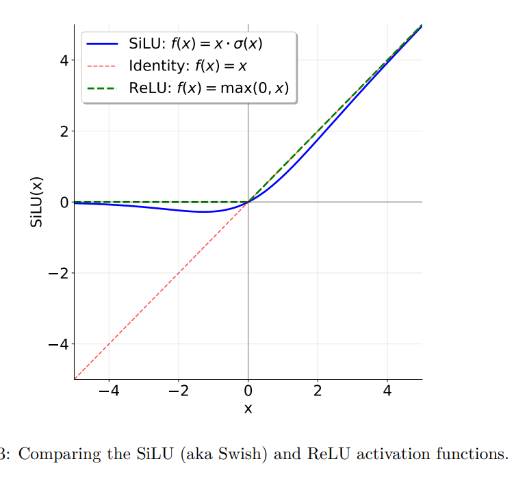
SiLU / Swish Activation Function
SiLU 是一种激活函数
\[\text{SiLU}(x) = x \cdot \sigma(x) = \frac{x}{1 + e^{-x}}\]SiLU 整体和 ReLU 差不多,主要区别是在 0 位置更平滑(可导)
Gated Linear Units (GLU)
GLU 的核心思想是使用门控机制来控制信息流动:
\[\text{GLU}(x, W_1, W_2) = \sigma(W_1 x) \odot W_2 x\]- $\sigma(W_1 x)$ 就是 $\frac{1}{1 + e^{-W_1 x}}$,会产生一个0到1之间的”门控(gate)信号”
- $W_2 x$ 表示进行线性变换
- $\odot$ 表示元素相乘:门控信号决定每个特征保留多少
- 当门控信号接近1时,特征几乎完全通过
- 当门控信号接近0时,特征被抑制
优点:传统的纯激活函数只能实现简单的分类(ReLU 过滤小于0的部分),GLU相当于为激活函数增加了一个可学习参数($W_1$),能根据不同的训练数据使用不同的过滤规则,相当于动态激活。$W_2$ 主要是为了增加一个线性特征,多一个可学习参数,提高表达能力。
缺点:GLU 相比于单纯的激活函数,参数量增加,计算量增加。
我们可以使用 SiLU 来代替原始 GLU 中的 $\sigma$ 激活函数(称为 SwiGLU),就能得到 FFN 的模型:
\[\text{FFN}(x) = \text{SwiGLU}(x, W_1, W_2, W_3) = W_2(\text{SiLU}(W_1 x) \odot W_3 x)\]其中:
- $x \in \mathbb{R}^{d_{\text{model}}}$
- $W_1, W_3 \in \mathbb{R}^{d_{\text{ff}} \times d_{\text{model}}}$
- $W_2 \in \mathbb{R}^{d_{\text{model}} \times d_{\text{ff}}}$,用于降维,让输出符合 FFN 要求,同时增加参数量。这个和传统的 FFN 是一样的 $\text{FFN}(x) = W_2(\text{ReLU}(W_1 x))$ (d → 4d → d)
- $d_{\text{ff}} = \frac{8}{3} d_{\text{model}}$,大于 $d_{\text{model}}$,实现维度的先扩展后压缩,提高计算时的表达能力(d → (8/3)d → d)
We offer no explanation as to why these architectures seem to work; we attribute their success, as all else, to divine benevolence.
作者自己也无法解释为什么 SwiGLU 更好,it just work
作业:Implement the SwiGLU feed-forward network, composed of a SiLU activation function and a GLU
1
2
3
4
5
6
7
8
9
10
11
12
13
14
15
16
17
18
19
20
21
22
23
24
25
26
27
def run_swiglu(
    d_model: int,
    d_ff: int,
    w1_weight: Float[Tensor, " d_ff d_model"],
    w2_weight: Float[Tensor, " d_model d_ff"],
    w3_weight: Float[Tensor, " d_ff d_model"],
    in_features: Float[Tensor, " ... d_model"],
) -> Float[Tensor, " ... d_model"]:
    """Given the weights of a SwiGLU network, return
    the output of your implementation with these weights.

    Args:
        d_model (int): Dimensionality of the feedforward input and output.
        d_ff (int): Dimensionality of the up-project happening internally to your swiglu.
        w1_weight (Float[Tensor, "d_ff d_model"]): Stored weights for W1
        w2_weight (Float[Tensor, "d_model d_ff"]): Stored weights for W2
        w3_weight (Float[Tensor, "d_ff d_model"]): Stored weights for W3
        in_features (Float[Tensor, "... d_model"]): Input embeddings to the feed-forward layer.

    Returns:
        Float[Tensor, "... d_model"]: Output embeddings of the same shape as the input embeddings.
    """
    w1x = einsum(w1_weight, in_features, "d_ff d_model, ... d_model -> ... d_ff")
    gate = w1x * torch.sigmoid(w1x)
    w3x = einsum(w3_weight, in_features, "d_ff d_model, ... d_model -> ... d_ff")
    gated = gate * w3x
    return einsum(gated, w2_weight, "... d_ff, d_model d_ff -> ... d_model")
Relative Positional Embeddings
在 Attention 操作中,我们希望 query 和 key 都携带位置信息(见 Positional Encoding),如果没有位置信息,这会带来语义理解问题:
- 输入1:狗追猫
- 输入2:猫追狗
这两个输入在模型看来是完全一样的,所以“猫”和“狗”哪个在前这个信息很重要
而输入的 token 是不带位置信息的,我们使用 Rotary Position Embeddings(RoPE) 来附加位置信息
对于序列中位置为 $ i $ 的token,将其查询向量 $ q^{(i)} $ 通过一个旋转矩阵 $ R^i $ 进行变换(q、k、v就是通过同一个 x 乘各自的权重得到的):
\[q'^{(i)} = R^i q^{(i)} = R^i W_q x^{(i)}\]其中 $R^i$ 是一个块对角矩阵:
\[R^i = \begin{bmatrix} R_1^i & 0 & 0 & \cdots & 0 \\ 0 & R_2^i & 0 & \cdots & 0 \\ 0 & 0 & R_3^i & \cdots & 0 \\ \vdots & \vdots & \vdots & \ddots & \vdots \\ 0 & 0 & 0 & \cdots & R_{d/2}^i \end{bmatrix}\]$R^i$ 中每个 0 是 2x2 矩阵:
\[\begin{bmatrix} 0 & 0 \\ 0 & 0 \end{bmatrix}\]$R^i$ 中每个 $R_k^i$($k \in {1, \ldots, d/2}$) 是:
\[R_k^i = \begin{bmatrix} \cos(\theta_{i,k}) & -\sin(\theta_{i,k}) \\ \sin(\theta_{i,k}) & \cos(\theta_{i,k}) \end{bmatrix}\]$R_k^i$ 是一个标准的旋转矩阵,假设我们有一个二维空间内的坐标 (x, y),我们将其绕 (0, 0) 旋转 $\theta$ 角度,可以表示为:
\[\begin{bmatrix} x' \\ y' \end{bmatrix} = \begin{bmatrix} \cos\theta & -\sin\theta \\ \sin\theta & \cos\theta \end{bmatrix} \begin{bmatrix} x \\ y \end{bmatrix}\]欧拉公式
复数 $z = a + bi$,可以表示为 $z = r(\cos\theta + i\sin\theta)$,证明略。得到欧拉公式 $e^{i\theta} = \cos\theta + i\sin\theta$,证明略。两个复数相乘可以得到新的复数:
\[(a + bi) \times (c + di) = (ac - bd) + (ad + bc)i\]令 $c = \cos\theta$, $d = \sin\theta$,$a = x$, $b = y$,等价于:
\[(x + yi) \times (\cos\theta + i\sin\theta) = (x\cos\theta - y\sin\theta) + (x\sin\theta + y\cos\theta)i\]结果是一个复数,用极坐标表示就是($x\cos\theta - y\sin\theta$, $x\sin\theta + y\cos\theta$),正好就是上面的矩阵运算后的结果,然后就能表示为:
\[x' + y'i = (x + yi) \times (\cos\theta + i\sin\theta) = (x + yi)e^{i\theta}\]用极坐标来表示就是:
\[\begin{bmatrix} x' \\ y' \end{bmatrix} = \begin{bmatrix} cos\theta \\ sin\theta \end{bmatrix} \times \begin{bmatrix} x \\ y \end{bmatrix}= e^{i\theta} \times \begin{bmatrix} x \\ y \end{bmatrix}\]也就是说欧拉公式可以实现极坐标上的点的旋转,旋转系数就是 $e^{i\theta}$,表示起来更简单,但是在数学上,和使用三角函数直接做旋转是一样的。
我们可以把这个坐标类比为 token 的 embedding 向量,每个 token 都有唯一的坐标。然后我们用旋转的角度将其类比于其位置,如果两个 token 的值相同,也就是坐标相同,但角度差距比较大,则说明它们离得就比较远。
我们将一个 embedding 向量($q^i$)的值,每两个组成一个 pair,也就是一个平面上的坐标(共 d/2 个平面),对每个 pair 都应用独立的旋转($R^i_k$),就会产生在 d/2 个平面维度上的旋转,也就是 $R^i$ 矩阵的作用。根据 i 也就是在句子中的位置的不同,旋转的角度 $\theta$ 也不同。这样我们就的在 d/2 个平面上各自旋转了向量的一部分,将位置信息嵌入了向量中。
人类理解相对位置时也使用多维度机制:
- 宏观:”这个词在文章开头提到”(低频)
- 中观:”这个词在前三段左右”(中频)
- 微观:”这个词就在这个逗号后面”(高频)
然后是计算旋转后的差异:
\[q' = (x_q cosθᵢ - y_q sinθᵢ, x_q sinθᵢ + y_q cosθᵢ)\] \[k' = (x_k cosθⱼ - y_k sinθⱼ, x_k sinθⱼ + y_k cosθⱼ)\] \[q'·k' = (x_q x_k + y_q y_k)cos(θⱼ - θᵢ) + (x_q y_k - y_q x_k)sin(θⱼ - θᵢ)\]通过点乘即可计算两个 token 的值差异以及位置差异。当然我们不会通过点乘显式计算差异,在后续的 attention 计算过程中会自然而然的去利用这些差异。
作业:: Implement a class RotaryPositionalEmbedding that applies RoPE to the input tensor
1
2
3
4
5
6
7
8
9
10
11
12
13
14
15
16
17
18
19
20
21
22
23
24
25
26
27
28
29
30
31
32
33
34
35
36
37
38
39
40
41
42
43
44
45
46
47
48
49
50
51
52
53
class Rope(torch.nn.Module):
    def __init__(self, theta: float, d_k: int, max_seq_len: int, device=None):
        '''
        Construct the RoPE module and create buffers if needed.
        Args:
            theta: float Θ value for the RoPE
            d_k: int dimension of query and key vectors
            max_seq_len: int Maximum sequence length that will be inputted
            device: torch.device | None = None Device to store the buffer on
        '''
        super().__init__()
        self.theta = theta # 注意 theta 是弧度,不是角度
        self.max_seq_len = max_seq_len
        self.d_k = d_k
        self.device = device
        freqs = 1.0 / (theta ** (torch.arange(0, d_k, 2).float() / d_k)) # (d_k/2, ),[θ^(0/d_k), θ^(-2/d_k), θ^(-4/d_k), ...]
        pos = torch.arange(max_seq_len, device=freqs.device).float() # (max_seq_len, ),位置序列,[0,1,2,...,max_seq_len-1]
        radians = einsum(pos, freqs, "pos, freqs -> pos freqs") # (max_seq_len, d_k/2),计算外积,得到每个位置的弧度列表
        self.cos = torch.cos(radians)  # (max_seq_len, d_k/2),注意参数不是角度,是弧度,半圆是pi
        self.sin = torch.sin(radians)  # (max_seq_len, d_k/2)

    def forward(self, x: torch.Tensor, token_positions: torch.Tensor) -> torch.Tensor:
        '''
        Process an input tensor of shape (..., seq_len, d_k) and return a tensor of the same shape.
        Note that you should tolerate x with an arbitrary number of batch dimensions. You should
        assume that the token positions are a tensor of shape (..., seq_len) specifying the token
        positions of x along the sequence dimension
        '''
        # 获取对应位置的cos和sin
        seq_len = x.size(-2)

        if token_positions is None:
            cos = self.cos[:seq_len]  # (seq_len, d_k/2)
            sin = self.sin[:seq_len]  # (seq_len, d_k/2)
        else:
            cos = self.cos[token_positions]  # (..., seq_len, d_k/2)
            sin = self.sin[token_positions]  # (..., seq_len, d_k/2)

        # 将输入向量分成两部分
        # x形状: (..., seq_len, d_k)
        x_reshaped = x.reshape(*x.shape[:-1], -1, 2)  # (..., seq_len, d_k/2, 2)
        x1 = x_reshaped[..., 0]  # (..., seq_len, d_k/2)
        x2 = x_reshaped[..., 1]  # (..., seq_len, d_k/2)

        # 应用旋转
        x1_rotated = x1 * cos - x2 * sin  # (..., seq_len, d_k/2)
        x2_rotated = x1 * sin + x2 * cos  # (..., seq_len, d_k/2)

        # 重新组合
        x_rotated = torch.stack([x1_rotated, x2_rotated], dim=-1)

        # 恢复原始形状
        return x_rotated.reshape(*x.shape)